Software, DSC Curve Solutions®, developed by CaoTechnology, represents a novel approach for thermal analysis that allows you to simulate DSC curves vividly for experiments under any conditions for a range of given thermal events; so that you can extract the sample properties by fitting DSC curves with DCS curves. This software is now available to all the thermal analysts and polymer scientists or engineers to advance thermal analysis and polymer science and technology.

How can DCS be useful?

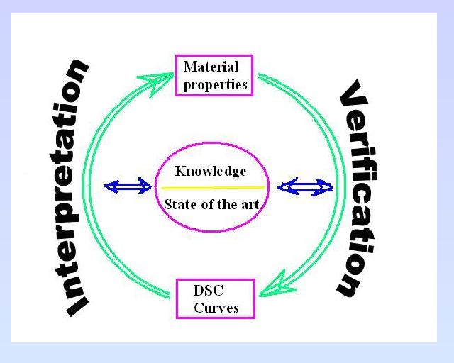
• It obtains sample thermal properties by fitting FULL DSC curves with DCS curves
— integrating interpretation and verification into one;
• It obtains all the relevant thermal properties from any single DSC run;
now you can determine curing and crystallisation kinetics from any single
non-isothermal DSC run;
• It covers a range of thermal events i.e. heat capacity, glass transition, enthalpy
relaxation, melting and crystallisation, curing and reactions; furthermore its
multi-component function allows you to deconvolute complex DSC curves readily;
• It solves your headache when observing a "shifting" "baseline" before and after an
endotherm or exotherm that makes your determination of the endotherm or
exotherm inaccurate and inconsistent. DCS tells you why the "baseline" "shifts"
and makes perfect fitting.
• It covers DSC runs under any experimental conditions e.g. linear heating, sinusoidal
(one or more frequencies) and/or saw-tooth modulation if you wish;
• It is a perfect aid to learn and teach DSC and polymers - you will have a better
understanding of the both.
• No training, no tutorial and no help would be needed, you'll become an instant
expert of DCS.

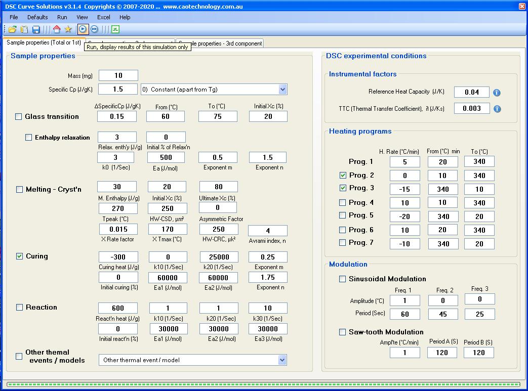
Screen shot of DSC Curve Solutions: check boxes of relevant thermal events and fill in your guess values, edit the heating program then click the run icon on the tool strip.

Definition of parameters used in DCS can be downloaded:

To have a free trial of DCS, simply click Free trial

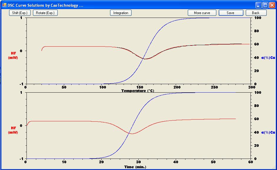
Determination of Thermal Transfer Coefficient:

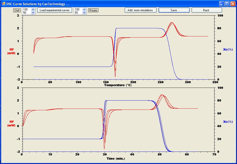
Jessica has obtained experimental DSC curves (shown in black) for a polymer material. She uses DCS to fit the DSC curves after inputting all the experimental conditions such as mass of the sample, heating rate etc. into DCS; she then A) adjusts the specific heat capacity to match the plateau of DCS curves with that of DSC's; B) tunes the thermal transfer coefficient, λ, which is an indicator of instrument performance, to fit the transient tail; C) finally she determines the melting thermodynamic parameters for the sample when she sees the curves are fitting to her satisfaction. In summary, by this DSC Curve Solutions curve fitting Jessica obtains:
Specific heat capacity: c_p = 2.03 J/Kg,
Melting peak temperature: T_m = 196°C,
Half width of the Gaussian crystallite size distribution: μ_m² = 250,
Asymmetric factor of the Gaussian crystallite size distribution = 0.03,
and the Thermal Transfer Coefficient: λ = 0.0031 J/Ks.

To have a free trial of DCS, simply click Free trial

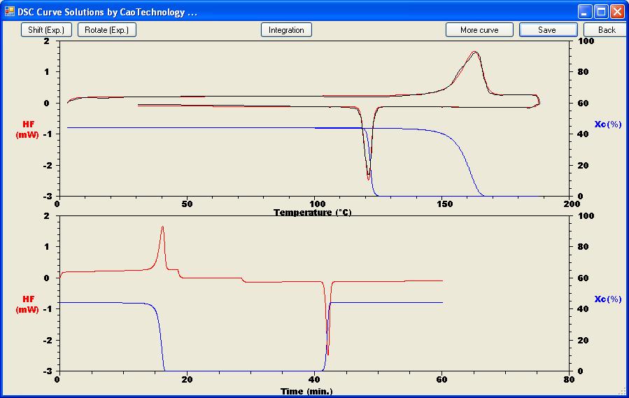
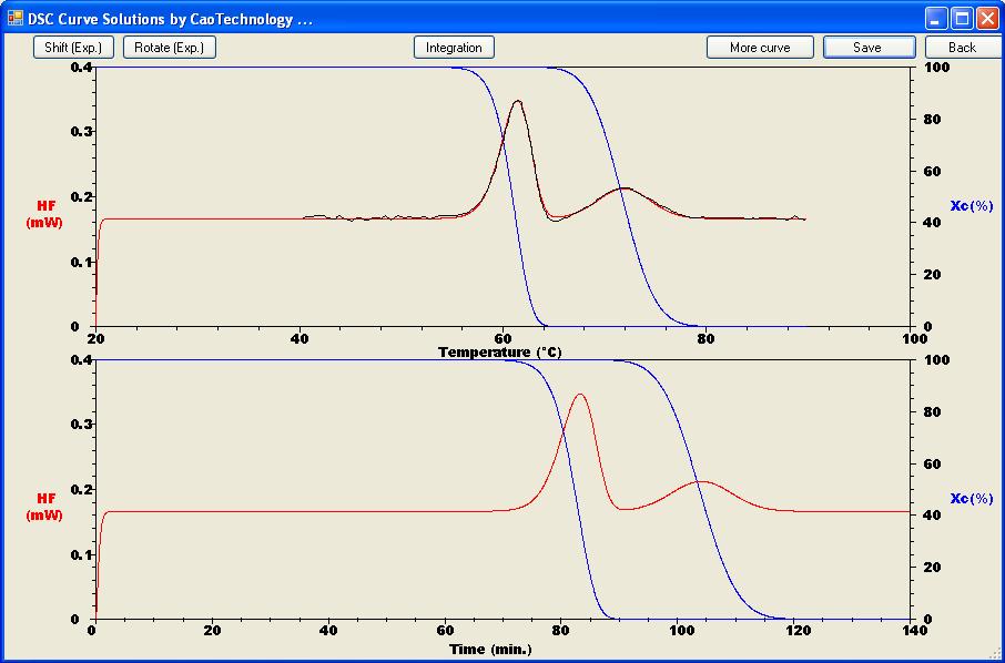
Polymer melting and crystallization:

An iPP sample was heated from 0°C to 190°C at 10°C /min, then stayed isothermally for 10 min, followed by a cooling at 5°C/min to 30°C, with its DSC curve shown in black line. After inputting all the known experimental parameters, one tuned relevant parameters to fit the DSC curve with the DCS curve to satisfaction, leading to determination of following parameters:
Specific heat capacity: c_p = 1.1 J/Kg at 0°C, ramping linearly towards 1.66 J/Kg at 200°C;
Melting enthalpy: ΔH = 95.22 J/g,
Melting peak temperature: T_m = 161.5°C,
Half width of the Gaussian crystallite size distribution: μ_m² = 65,
Asymmetric factor of the Gaussian crystallite size distribution = -0.06,
Crystallisation rate factor: A_k = 0.024,
Maximum crystallisation rate temperature: T_max = 118.5;
Half width of the crystallisation rate distribution: μ_k² = 95;
and Avrami index: n = 4.
Furthermore, assuming the melting enthalpy, ΔH for 100% crystallised iPP is 207 J/g,
one obtains the crystallinitity curve as well.

To have a free trial of DCS, simply click Free trial

Protein denaturazation:

The DSC curve for a multi-domain immunoglobulin G (IgG) protein shows two denaturazation (melting) endotherms slightly overlapping (black curve). Using DCS, Veronica readily deconvoluted the DSC curve and obtained following parameters:
Domain 1: Denaturation enthalpy: ΔH = 12.5 J/g,
Peak temperature: T_m = 61.2°C;
Half width of the Gaussian distribution, μ_m² = 12,
Asymmetric factor of the Gaussian distribution = -0.065,
Domain 2: Denaturation enthalpy, ΔH = 5.4 J/g;
Peak temperature: T_m = 71.7°C,
Half width of the Gaussian distribution, μ_m² = 37,
Asymmetric factor of the Gaussian distribution = 0.

To have a free trial of DCS, simply click Free trial

Epoxy curing:

Adam wants to known the kinetic parameters for an epoxy resin. He heats the epoxy to 290°C at 5°C/min, and obtains curing exotherm DSC curve shown in black. Using the autocatalytic model, Adam readily determines the kinetic parameters of the epoxy resin by fitting this SINGLE run DSC curve (black) with the DCS curve (red) to satisfaction.
Curing enthalpy: ΔH = -205 J/g;
Frequency factor: k₁₀ = 0 (Activation energy, E_a1, can be any in this case);
Frequency factor: k₂₀ = 12200 s^-1;
Activation energy: E_a2 = 51450 J/mol;
Exponent: m = 0.60
Exponent: n = 1.45

Thus, Adam obtains all the parameters describing the curing behaviour of the epoxy resin, no more no less:

$$ \frac{d \alpha}{dt} = 12200 \;\; exp \left ( \frac{-51450}{R \, T} \right ) \; \alpha ^{0.6} \; (1-\alpha)^{1.45} $$

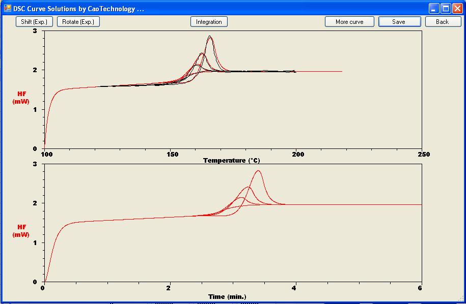
Enthalpy relaxation:

James has obtained a group of enthalpy relaxation DSC curves (shown in black) for a polymer material, with the quenched and that after 30, 200 and 2000 min. ageing being shown in the figure. He then uses DCS to fit the DSC curves using following paramters:
Relaxation enthalpy: ΔH = 5.7 J/g;
Frequency factor: k₀ = 1.25 s^-1;
Activation energy: E_a = 380 J/mol;
Exponent: m = 0.50;
Exponent: n = 0.5
In particularly, James has amazingly found the four DSC curves correspond to 100%, 75%, 40, and 0% degree of relaxation respectively (or 0%, 25%, 60% and 100% degree of ageing).

To have a free trial of DCS, simply click Free trial

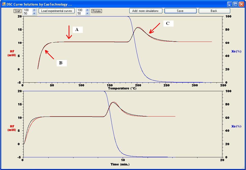
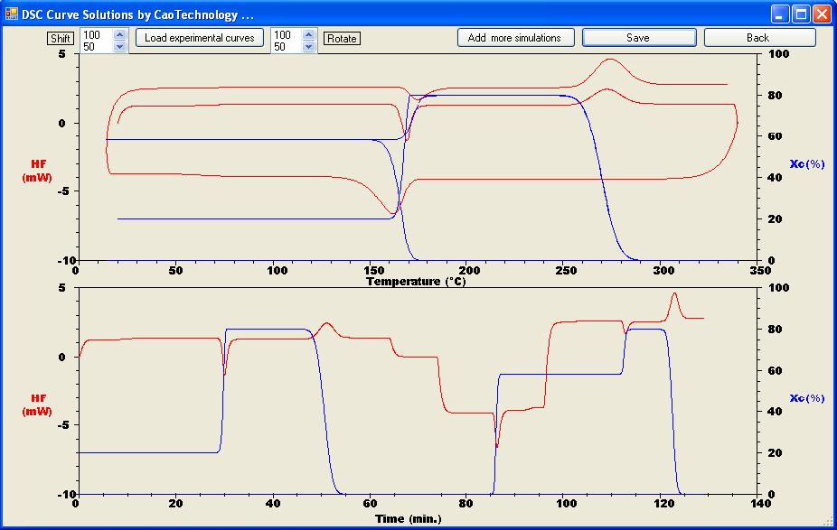
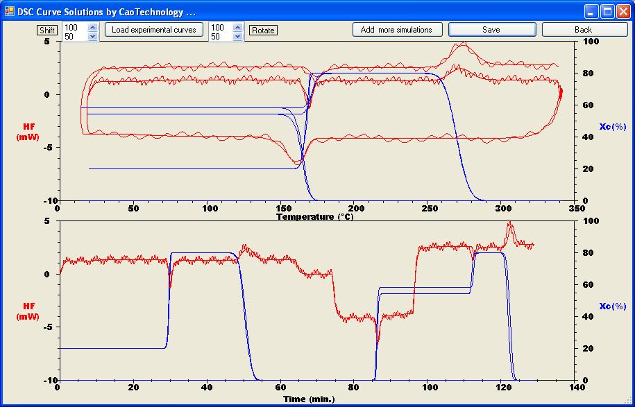
DSC Curve simulation for melting and crystallization:

Catherina has a semi-crystalline polymer with 20% initial crystallinity and the ultimate crystallinity being 80%. She runs DSC experiment at 5°C/min from 20°C to 340°C, holds isothermally for 10 min, cools down to 10°C at 15°C/min and finally heats it up to 340°C at 10°C/min. She obtains the numerical experimental DSC curve and the crystallinity curve as follows:

To have a free trial of DCS, simply click Free trial

DSC curve simulation for modulation:

Peter is an instrumentalist interesting in temperature modulation. He runs Catherina's experiment with a sinusoidal modulation with amplitude and period being 1.0°C and 45 seconds respectively. He further superimposes a saw-tooth modulation with amplitude and period being 1.0°C/min and 240 seconds on the sinusoidal modulation. He obtains following DSC curves (Catherina's curves shown in Example 2 are superimposed in the screenshot.

To have a free trial of DCS, simply click Free trial

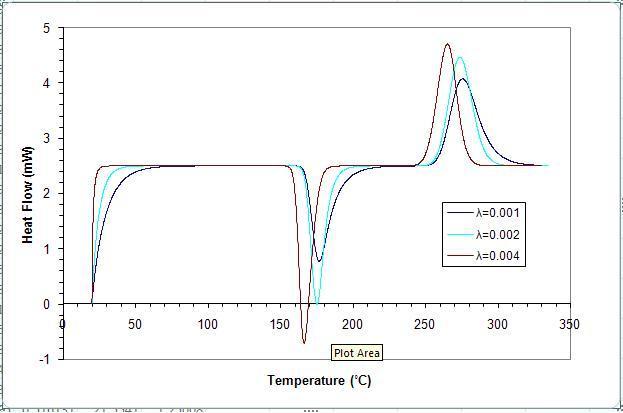
DSC curve simulation for instrument factor:

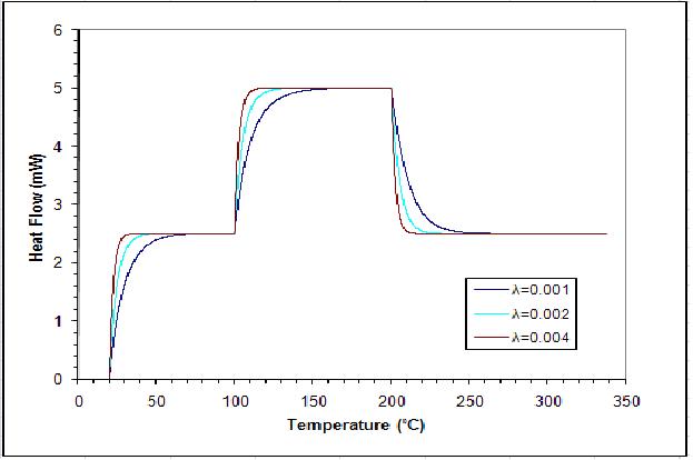
DSC has been working for Steve years and years. Steve wants now to show how the Thermal Transfer Coefficient (TTC), λ, has been working for DSC. He runs 3 simulations with different λ values for a given sample under a given set of DSC conditions. As shown in the following figure, the DSC curves vary with λ due to the intrinsic transient effect of DSC measurements that is undesirable. Steve further assumes a sample with step up and a step down changes in its specific heat capacity over a temperature range. He obtains the numerical experimental DSC curves shown below. Steve thus concludes a high λ is desirable to obtain DSC curves with less distortion.

To have a free trial of DCS, simply click Free trial

Q: What is the key performance indicator of a DSC instrument ?
A: Higher λ — The shorter the starting tail, the better the DSC instrument is !

DSC curve simulation for effect of pan:

Similar to Steve, Fiona wants to examine the effect of reference heat capacity, i.e. the DSC cell pans. She has obtained the numerical experimental DSC curves as follows. What do these curves tell us ?

To have a free trial of DCS, simply click Free trial

Differential Scanning Calorimetry (DSC):

Differential scanning calorimetry, or DSC, is an analytical thermal analysis methodology that measures heat flow required to scan temperature in a predetermined manner, while the heat flow is quantified as a relative value over a reference with known stable thermal properties. Application of this differential technique represents a great advance in calorimetry. DSC is widely used in materials in particular polymer analysis.

Glass transition:

Glass transition, aka glass-liquid transition, glass temperature, is a reversible transition in amorphous materials (or amorphous region in a material) from glassy state to rubbery state as temperature increases. Glass transition is the most important characteristic of polymer materials.

Avrami equation:

The Avrami equation is an equation describing how crystallinity of a material progresses with time at constant temperatures:

$$ \alpha = 1- exp \left (-k \, t^n \right ) $$

where, α — degree of crystallinity; t — time; k — rate constant (a positive number); n — Avrami index, which is an indicator of nucleation mechanism.

To learn the theory of DSC Curve Solutions (DCS ®), click the link for references shown in naviation bar.